Re-coding Categorical Variables in R
While I have done data analysis almost exclusively in R for most of my career, until recently I have done a lot of my data cleaning in Stata. I have even told people in the past that I though Stata was better at data cleaning than R. However, when I switched my graduate statistics class from Stata to R last year, I decided that I needed to teach my students how to clean data in R. True to the old saying, there is no better way to learn than teach. In this case, I realized that my attitude toward data cleaning in R was more about my lack of familiarity with some nice utilities in R than it was about R itself.
In this post, I wanted to use some code from one of my current projects to outline how to efficiently re-code categorical variables in R. I will first outline how I used to do it and then demonstrate much simpler code to achieve the same effect. I am not using any additional packages here, including the tidyverse. All code is base R.
The Data
The data I am using come from a data extract of the General Social Survey (GSS). I am particularly interested in the variable PRAY in this dataset. Yes, the GSS capitalizes all of its variable names because REASONS. You can access the CSV data here.
gss <- read.csv("gss_relig.csv")
table(gss$PRAY)
##
##     0     1     2     3     4     5     6     8     9
## 28232  9065  9936  4099  2321  5469  2239    96   302
The default data came in numeric format. The online codebook for the GSS tells me that these numeric codes correspond to the following categories.
| Numeric Code | Category |
|---|---|
| 0 | Not applicable |
| 1 | Several times a day |
| 2 | Once a day |
| 3 | Several times a week |
| 4 | Once a week |
| 5 | Lt once a week |
| 6 | Never |
| 8 | Don’t know |
| 9 | No answer |
Ultimately, I want to turn these numeric codes into a proper factor variable. There are several issues to consider before proceeding:
- There are multiple missing value codes to enter (0,8,9)
- The numbering is the reverse of how I want the ordinal variable coded. I want higher values to indicate higher frequency of prayer.
- Most importantly, the category of “Never” was not given as an explicit option until 2004, so I can’t compare data across time very well with that category. Therefore, I want to collapse the “Never” and “Lt once a week” category together.
My Old Approach
My old approach to handling this sort of re-code problem would have been to apply what I call the bracket and boolean approach. Here is what that code would look like:
gss$pray <- NA
gss$pray[gss$PRAY==5 | gss$PRAY==6] <- "lt once a week"
gss$pray[gss$PRAY==4] <- "once a week"
gss$pray[gss$PRAY==3] <- "several times a week"
gss$pray[gss$PRAY==2] <- "once a day"
gss$pray[gss$PRAY==1] <- "several times a day"
gss$pray <- factor(gss$pray)
gss$pray <- relevel(gss$pray, "several times a day")
gss$pray <- relevel(gss$pray, "once a day")
gss$pray <- relevel(gss$pray, "several times a week")
gss$pray <- relevel(gss$pray, "once a week")
gss$pray <- relevel(gss$pray, "lt once a week")
table(gss$pray, gss$PRAY, exclude=NULL)
##
##                            0     1     2     3     4     5     6     8     9  <NA>
##   lt once a week           0     0     0     0     0  5469  2239     0     0     0
##   once a week              0     0     0     0  2321     0     0     0     0     0
##   several times a week     0     0     0  4099     0     0     0     0     0     0
##   once a day               0     0  9936     0     0     0     0     0     0     0
##   several times a day      0  9065     0     0     0     0     0     0     0     0
##   <NA>                 28232     0     0     0     0     0     0    96   302     0
First, I created a new variable full of missing values. I then used indexing and boolean statements to replace those missing values with character strings of the correct categories. I then had turned those character string into a factor with the factor command. However, by default, that command will order my categories alphabetically, so I then ran five relevel commands to get the ordering correct. I then run a table command with the exclude=NULL option to include missing values to check myself before I wreck myself. It works, but I am not proud of that code.
Had I bothered to read the help file for factor, I would have realized that I could actually specify ordering of the categories with the levels argument, so I could have simplified my code a little bit by removing the factor and relevel commands and replacing them with the following:
gss$pray <- factor(gss$pray,
                   levels=c("lt once a week","once a week",
                            "several times a week","once a day",
                            "several times a day"),
                   ordered=TRUE)
The ordered option is particularly useful here for running greater than or equal to booleans on factor variables, as I will demonstrate below. Using this code will improve my initial code considerably, but I can still do much better.
My New Approach
My new approach takes advantage of two functions. First, the factor function itself is very flexible and can often be used to recode categorical variables without resort to the bracket and boolean approach. In this case, I can take advantage of the levels and labels argument to directly code my original numeric variable into a categorical variable in one line.
The second function that is essential to date cleaning in R is the ifelse command. This function takes a boolean statement and assigns the value in the second argument if TRUE, and the value in the third argument if FALSE. In this case, I can easily combine the 5 and 6 numeric values from the original variable into just the value of 5 with:
ifelse(gss$PRAY==6, 5, gss$PRAY)
To do the entire re-coding in one line, I just need to wrap a factor function around that code as follows:
gss$pray <- factor(ifelse(gss$PRAY==6, 5, gss$PRAY),
                   levels=5:1,
                   labels=c("lt once a week","once a week",
                            "several times a week","once a day",
                            "several times a day"),
                   ordered = TRUE)
table(gss$pray, gss$PRAY, exclude=NULL)
##
##                            0     1     2     3     4     5     6     8     9  <NA>
##   lt once a week           0     0     0     0     0  5469  2239     0     0     0
##   once a week              0     0     0     0  2321     0     0     0     0     0
##   several times a week     0     0     0  4099     0     0     0     0     0     0
##   once a day               0     0  9936     0     0     0     0     0     0     0
##   several times a day      0  9065     0     0     0     0     0     0     0     0
##   <NA>                 28232     0     0     0     0     0     0    96   302     0
Just like that, twelve lines of code become one.
You can apply this same trick to data to re-code and collapse data that is already coded as a factor variable. You just need to use cascading ifelse command to collapse and use a character vector for the levels.
To demonstrate, I use my new pray variable to create a pray.simple variable that collapses the data as follows:
- “lt once a week”
- “weekly”: “once a week” and “several times a week”
- “daily”: “once a day” and “several times a day”
I can do this again in a single line of code by using cascading ifelse statements. When the result of an ifelse statement is FALSE, I use another ifelse statement to continue looking for categories that I need.
gss$pray.simple <- factor(ifelse(is.na(gss$pray), NA,
                                 ifelse(gss$pray>="once a day", "daily",
                                        ifelse(gss$pray>="once a week",
                                               "weekly", "lt once a week"))),
                          levels=c("lt once a week", "weekly", "daily"),
                          ordered=TRUE)
table(gss$pray, gss$pray.simple, exclude=NULL)
##
##                        lt once a week weekly daily  <NA>
##   lt once a week                 7708      0     0     0
##   once a week                       0   2321     0     0
##   several times a week              0   4099     0     0
##   once a day                        0      0  9936     0
##   several times a day               0      0  9065     0
##   <NA>                              0      0     0 28630
The first ifelse command filters out the missing values. Then I can use >= booleans (because I used the ordered=TRUE on the factor variable) to partition my valid categories and collapse them into the three that I want. I then define the ordering of the categories by feeding a character vector into levels. The table command shows that everything is ended up where I expected it to be.
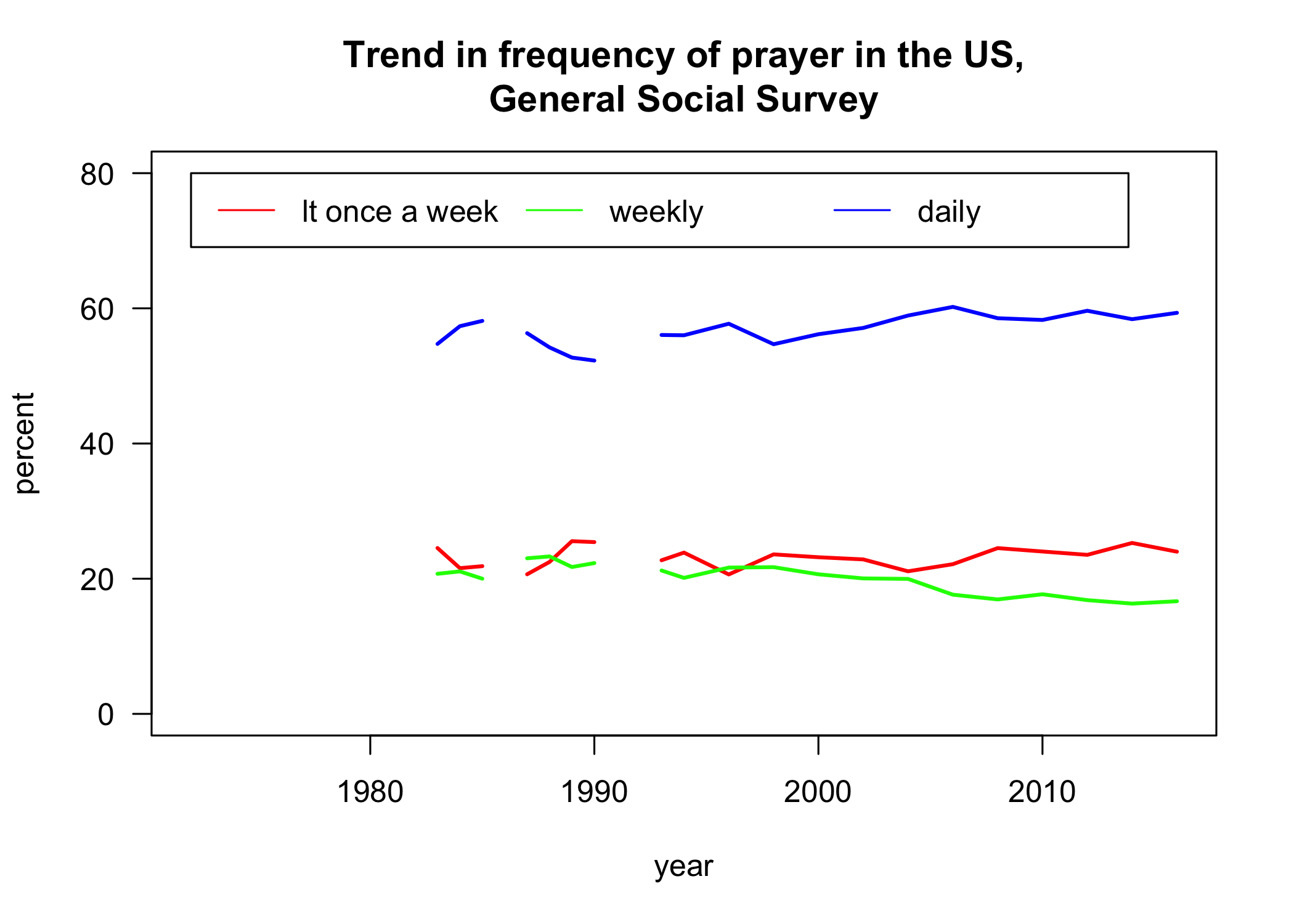
Now that my variable is all coded properly, I can look at the trend over time in the frequency of prayer:
p <- prop.table(table(gss$YEAR, gss$pray.simple),1)
matplot(as.numeric(rownames(p)), 100*p, type="l", lty=1, col=rainbow(3),
        lwd=2, las=1, ylab="percent", xlab="year", ylim=c(0,80),
        main="Trend in frequency of prayer in the US,\nGeneral Social Survey")
legend(1972, 80, legend=levels(gss$pray.simple), lty=1, col=rainbow(3),
       ncol=3)